
My name is Anton Kazakov. I am a Java developer with 7 years of backend development experience. In this article, I am going to tell you about one of my pet projects using machine learning. The goal of the project was to get familiar with model training, data preparation and predict phase. Today I will share my process and results, to hopefully teach and inspire others.
The main idea is to collect gyroscope data from a smartwatch during a workout. After the workout is finished, a person can use a smartphone to create a workout journal, where they can search for and find all the gym activities undertaken during the workout with details like reps.
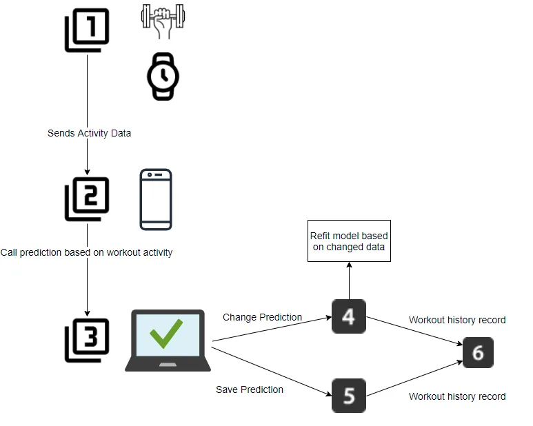
Flow Diagram
1.1
The data is a dummy csv file with gyroscope coordinates and the type of activity. 3 people did 3 types of exercises: situps, abs, pullups and we marked this type. So it will be my test and training data.
1.2
Data preparation: features, train data.
To use the data with the keras model I did some pre-processing to match keras to the expected input.
First I mapped features into numbers, then shuffled and split the data into test and model-fit sets.
There are several types of machine learning models, I consider here two types: learning with a ‘teacher’ (supervised) – when we already have samples for the model, and unsupervised, when we do not have such samples and we want our model to find all the dependencies in our data.
I used LabelBinarizer to create biriez targets. LabelBinarizer is an SciKit Learn class that accepts Categorical data as input and returns an Numpy array.
1.3
I used the keras framework to build custom models. Keras is basically a wrapper around TensorFlow. The sequential API allows you to create models layer-by-layer for most problems. It is limited in that it does not allow you to create models that share layers or have multiple inputs or outputs.
Alternatively, the functional API allows you to create models that have a lot more flexibility as you can easily define models where layers connect to more than just the previous and next layers. In fact, you can connect layers to (literally) any other layer. As a result, creating complex networks such as siamese networks and residual networks becomes possible:
model = models.Sequential()

model.add(layers.Conv1D(32, 3, activation=’relu’,
input_shape=(None, train_data.shape[-1])))
model.add(layers.MaxPooling1D(2))
model.add(layers.Conv1D(32, 3, activation=’relu’))
model.add(layers.GlobalMaxPooling1D())
model.add(layers.Dropout(0.2))
model.add(layers.Dense(32, activation=’relu’))
model.add(layers.Dense(test_labels.shape[-1], activation=’softmax’))
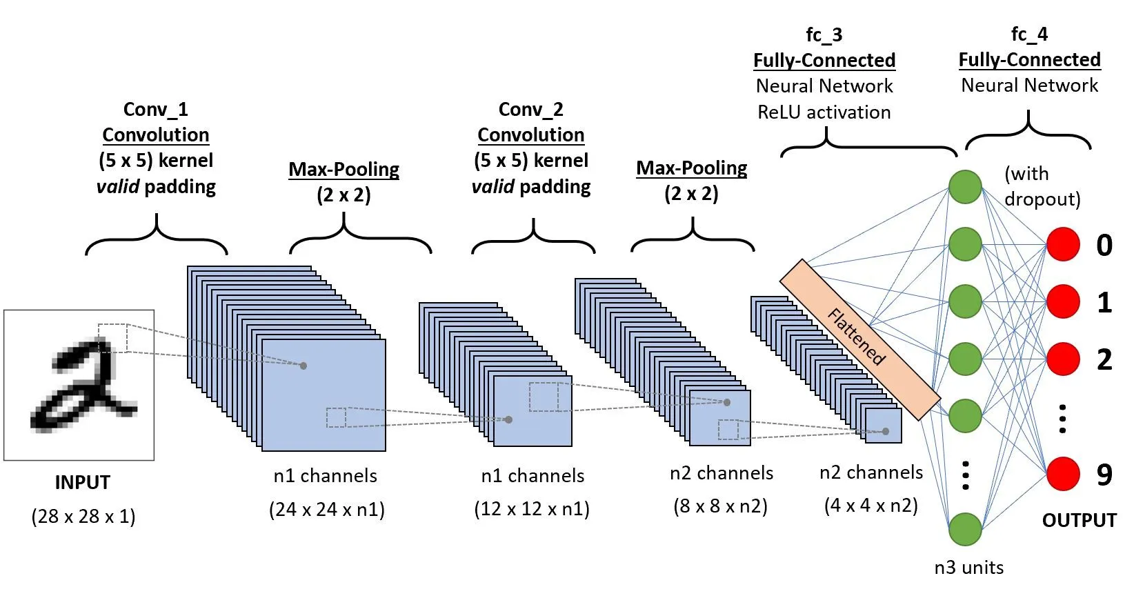
The first layer will be a convolution with a “relu activation” function. The convolutional neural network, or CNN for short, is a specialized type of neural network model designed for working with two-dimensional image data, although they can be used with one-dimensional and three-dimensional data.
In the context of a convolutional neural network, a convolution is a linear operation that involves the multiplication of a set of weights with the input, much like a traditional neural network. Given that the technique was designed for two-dimensional input, the multiplication is performed between an array of input data and a two-dimensional array of weights, called a filter or a kernel.
The Activation function relu is commonly used and it’s responsible for normalizing the data.
MaxPooling1D(2) layer is a customizable model for 2 dimension data. Next is the convolution layer with GlobalMaxPooling.
Then we use a Dense layer to feed all the outputs from the previous layer to all its neurons.
Dropout layers are used to prevent overfitting and the dense layer feeds the all outputs from the previous layer to all its neurons. The Softmax activation function is used for predicting probabilities for each workout activity.
1.4
OK now that I’ve prepared all the data from the csv files, let’s go step by step through the compile and fit processes.
Compile defines the loss function, the optimizer and the metrics. That’s all. It has nothing to do with the weights and you can compile a model as many times as you want without causing any problem to pretrained weights. You need a compiled model to train (because training uses the loss function and the optimizer).
The Loss function I’m using is MSE (Mean Square Error). It’s a method of evaluating how well a specific algorithm models the given data.
loss = square(y_true – y_pred)Accuracy is one metric for evaluating classification models. Informally, accuracy is the fraction of predictions our model got right. Formally, accuracy has the following definition: Accuracy = Number of correct predictions Total number of predictions.
1.5
Now we get to show the charts and compiled model. The last step is evaluation. I can see that the success rate is almost 1, 0.996. We have good guessing since the probability we have with the result is a little bit smaller than 1. The final step is to predict on some test value, so the probability for 5-th of activity is almost 1, so it is a very good score. There is much more I could do from here but am happy to share progress on this so far.
Make sure to check out the video demonstration. Good luck with your own pet projects. If you would like our support with a ML project, let’s talk.